
AI in Colombian container terminals, more than a buzzword
After writing a series of articles on how to apply IA to recruiting, I decided it was time to take a break and change the topic of my articles (at least temporarily).
For me, one of the most interesting and practical applications of ML is fraud detection in financial transactions, a field that can be approached from classification models or anomaly detection analysis.
In general, exploring and experimenting with fraud detection models is somewhat more complex due to the lack of publicly available datasets. This is understandable, as few financial institutions are willing to expose potentially sensitive financial and operational information to the public domain.
The objective of this article is to present a simple approach to the problem of fraud detection, which I hope will serve as either an initial reference or a starting point for developing more complex models.
This project is based on a synthetic dataset created by PaySim, which has generated a dataset from private real-world transactions of a mobile money service implemented in an African country. The synthetic dataset simulates normal transactional operations, into which malicious behavior has been injected to evaluate the performance of fraud detection models. The original dataset is available on the Kaggle platform (https://www.kaggle.com/ntnu-testimon/paysim1).
The code for this project can be found at:
https://github.com/ortizcarlos/fraud_detection/blob/master/Financial%20fraud%20detection.ipynb
Let’s start by exploring the data to gain an understanding of key information such as dataset size, columns, missing data, outliers, etc.

The dataset is moderately large with 6,362,620 rows and 11 columns.
step — maps a unit of time in the real world. In this case 1 step is 1 hour of time. Total steps 744 (30 days simulation).
type — CASH-IN, CASH-OUT, DEBIT, PAYMENT and TRANSFER.
amount — amount of the transaction in local currency.
nameOrig — customer who started the transaction
oldbalanceOrg — initial balance before the transaction
newbalanceOrig — new balance after the transaction
nameDest — customer who is the recipient of the transaction
oldbalanceDest — initial balance recipient before the transaction. Note that there is not information for customers that start with M (Merchants).
newbalanceDest — new balance recipient after the transaction. Note that there is not information for customers that start with M (Merchants).
isFraud — This is the transactions made by the fraudulent agents inside the simulation. In this specific dataset the fraudulent behavior of the agents aims to profit by taking control or customers accounts and try to empty the funds by transferring to another account and then cashing out of the system.
isFlaggedFraud — The business model aims to control massive transfers from one account to another and flags illegal attempts. An illegal attempt in this dataset is an attempt to transfer more than 200.000 in a single transaction.
‘PAYMENT’, ‘TRANSFER’, ‘CASH_OUT’, ‘DEBIT’, ‘CASH_IN’
Distribución por tipo de transacción (type)
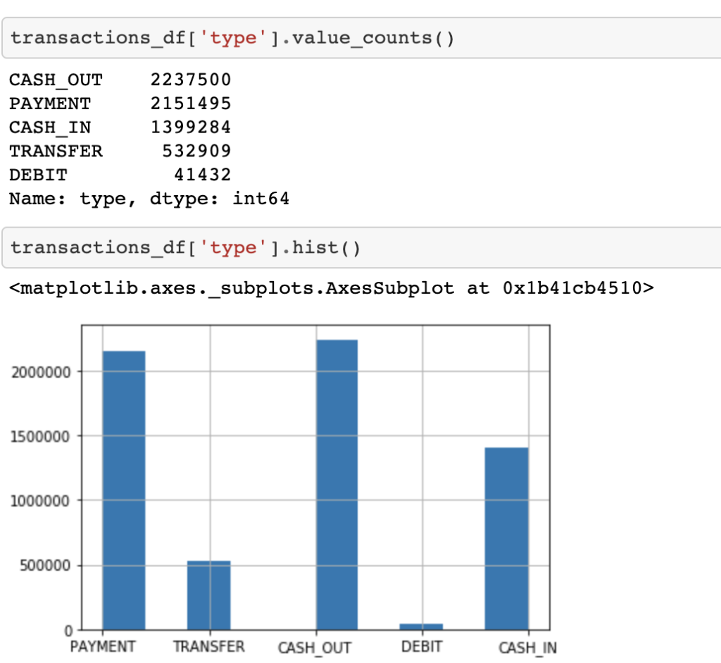
Let’s see how many frauds we have.
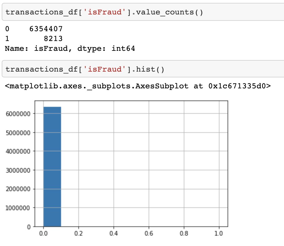
Only 8,213 rows out of a total of just over 6 million represent frauds (only 0.13%!). This is almost to be expected, as generally in a financial dataset, the number of fraudulent samples is almost always very small compared to the total number of transactions.
This class imbalance (frauds represent only 0.13% of the total) is a very important factor to consider when building our model.
Now, let’s see how many frauds there are by transaction type:
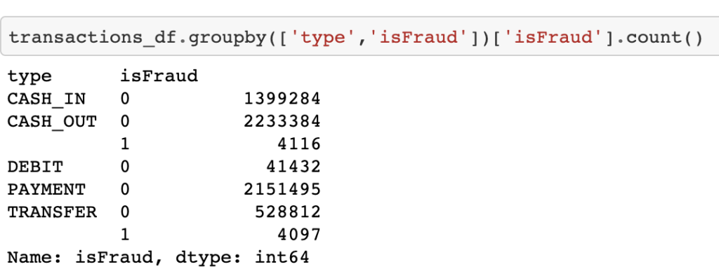
According to the data, frauds have only occurred in CASH_OUT and TRANSFER transactions.
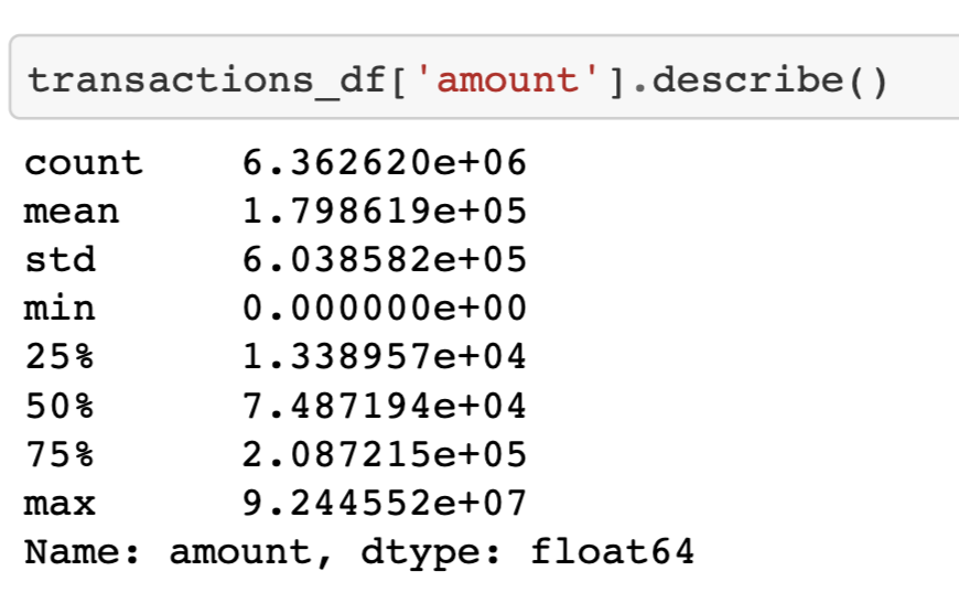
Let’s visualize histograms of the transaction amount by transaction type (type), trying to identify any patterns in the data.

The previous histograms show that for all cases, the data is concentrated on the left with very marked outliers in the CASH_OUT and TRANSFER transaction types, which are exactly the types of transactions where we have frauds. Let’s see if visualizing the interquartile range of the data reveals something more interesting.

Let’s now visualize the distribution of the amount in fraudulent transactions.
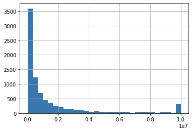
The histogram of the frauds also shows that the data is concentrated on the left (positive skew) and outliers at 10M.
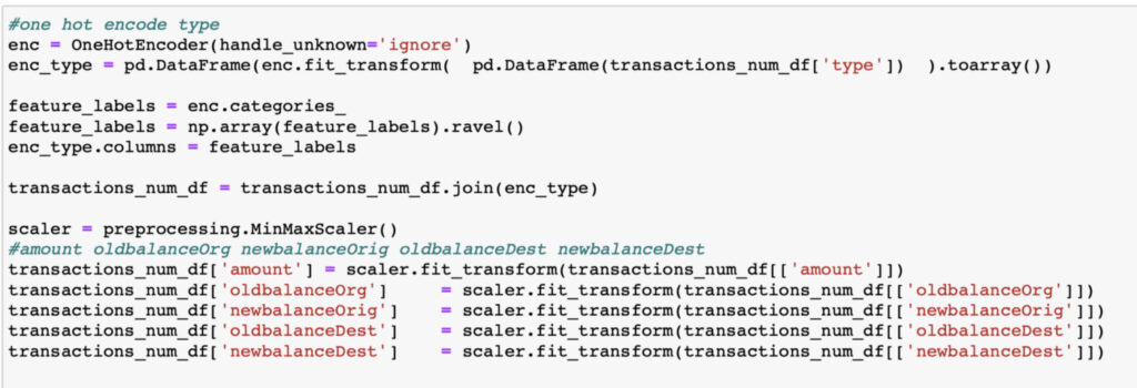
Let’s start with the conversion of the ‘type’ column, which is categorical, with the values (‘PAYMENT’, ‘TRANSFER’, ‘CASH_OUT’, ‘DEBIT’, ‘CASH_IN’).
For the ‘type’ column, one could consider an ordinal representation such as 1 = PAYMENT, 2 = TRANSFER, 3 = CASH_OUT, and so on. However, this might lead the model to learn that PAYMENT and TRANSFER are more similar than DEBIT and CASH_IN, when in reality there is no ordinal relationship between them. Therefore, it’s better to perform a One Hot Encoding.
Let’s now look at the correlation of all the columns in the dataset with respect to the label (isFraud), which is the value our model should be able to predict.
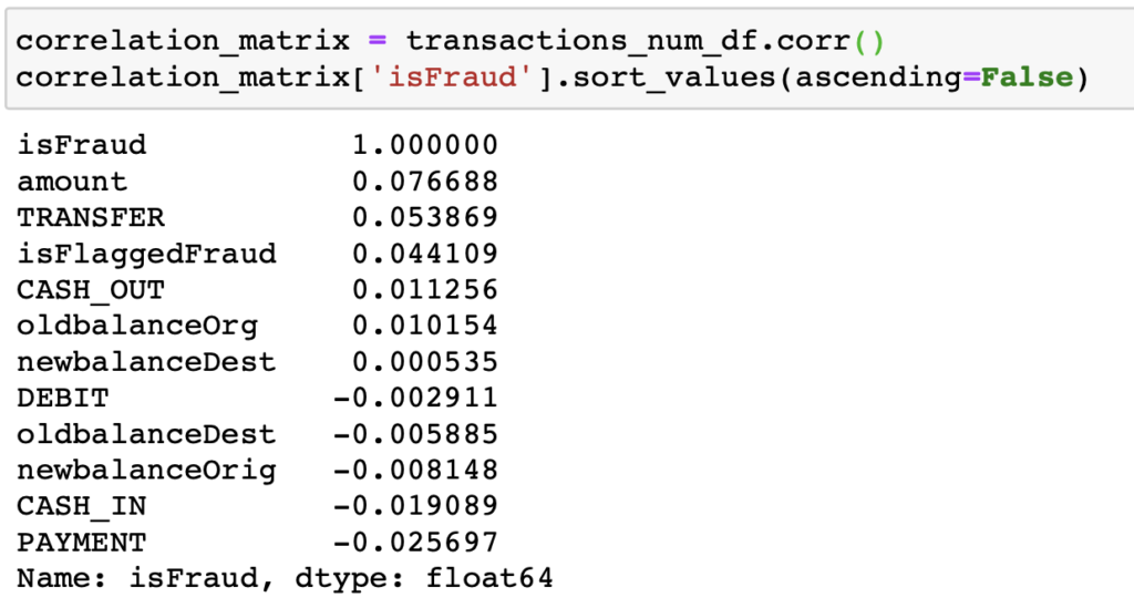
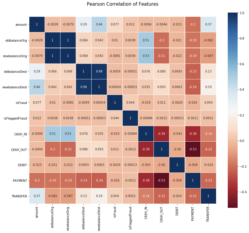
We can observe that the columns most correlated with the isFraud label are:
Positively: amount, TRANSFER, isFlaggedFraud, CASH_OUT, oldbalanceOrg
Negatively: PAYMENT and CASH_IN (precisely, there are no frauds for these types of transactions).
Before splitting the dataset into training and testing, it is important to find a splitting method that is more effective for the model than a purely random one. In this case, since we have so few records indicating fraud, it would be beneficial for the training and testing datasets to have an equal proportion of rows with frauds. This type of split is called stratified splitting, and for this, we will use StratifiedShuffleSplit from scikit-learn.
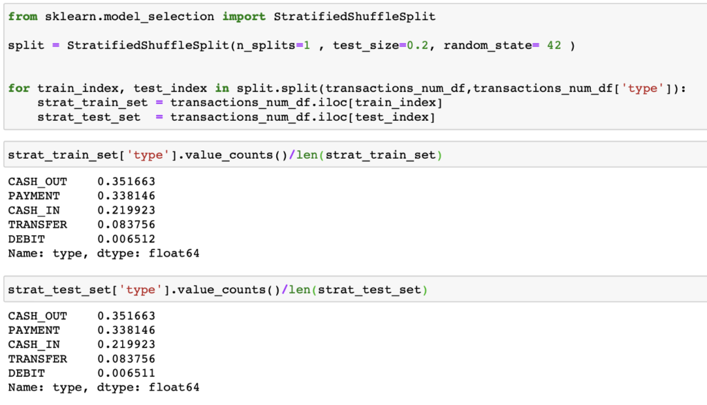
Let’s start by creating a model based on the Random Forest algorithm, which is a flexible and easy-to-use algorithm that produces good results even without tuning the hyperparameters. Additionally, it is useful for handling large datasets with many features, although this particular dataset is not that large.

After training the model, we found Wow!, an accuracy of 99.99%! But… not so fast! Let’s not be dazzled by that value. Remember that the number of rows with frauds represents ONLY 0.13% of the total, so an accuracy of 99.99% could just be telling us that our model is excellent at predicting NON-fraudulent transactions 🙂
For classification models, there are more suitable metrics to evaluate performance, including the confusion matrix and precision and recall. When our model predicts a fraud, precision tells us the percentage of accuracy with which it did so. Meanwhile, recall (also known as sensitivity or completeness) tells us what percentage of the total frauds our model is able to identify.
First, we calculate the confusion matrix, where we obtain: TP: true positives, FP: false positives, TN: true negatives, and FN: false negatives. With these, we calculate precision and recall.

The results are still very good! We have a precision of 100% and a recall of 91.64%!
This means that our model is able to recognize 91.64% of the frauds, and when it predicts a fraud, it does so with 100% accuracy!
However, we must be cautious and ensure that the good values of these metrics are not simply due to the model overfitting the training data…
To ensure that the model’s performance is as good as the previous metrics suggest, let’s implement a mechanism called cross-validation. This basically involves splitting the training dataset into k smaller data blocks (folds), and with each of these:

After writing a series of articles on how to apply IA to recruiting, I decided it was time to take a break and change the topic of my articles (at least temporarily).

After writing a series of articles on how to apply IA to recruiting, I decided it was time to take a break and change the topic of my articles (at least temporarily).